Blog, Elementor, Marketing, Mortgage Broker Website, WordPress, WordPress Shortcode, Yabber

Website ABS Census API and Website Graphs

This article is intended for clients, and it provides an update to the core Saturn functionality that'll be introduced to each website by default in the near future. In light of the ridiculous success the Saturn program has enjoyed, we're building in core location-based data into the back of the mortgage broker website framework delivered to brokers, and it's expected that this resource will be developed into your Saturn module when you choose to incorporate that program into your business. Other reasons for integration of the geographic information into broker websites is to support the forthcoming inclusion of property listings that'll be used to support your property partners, and to leverage your continued content creation programs.

A part of the data used to support your geographic (Saturn) pages is the Australian Census data, and this functionality is served via a RESTful API that returns all datasets made available via the Australian Bureau of Statistics. Most of our brokers would be familiar with the data as it's used as a core source of information when building profiles for advertising, but few would be familiar with the API and graphing tools made available to them by virtue of their standard Yabber access. In this article we'll touch on the very basics of the API, although we expect to have full documentation made available in coming months that'll expose you to the millions of records and thousands of graphing options made available via this vital source of data.

Note: It's likely that your aggregator will already supply demographic-based research tools, including their own version of the Census data. Our difference is that the information is designed to be directly integrated with your website and other marketing efforts. Note that any self-respecting marketing group will likely offer their own equivalent API.

The graphs on this page are very limited examples. There are literally millions of permeations of graphs, and part of the reason we're delaying more advanced features, including a broader release of the only Census Elementor plugin the country, is because we're looking at more efficient ways of making any graph available to you by way of custom fields - a very frustrating strain on our fuzzy brains (at the moment a facility to limit fields returned is not implemented).

Example Graphs

Basic gaphing is returned to a page with the required attributes of type and code, with the type denoting what graph is to be returned, and the code specifying what statistical region(s) that should be queried. Other attributes are necessary for more advanced graphing, such as the fields attribute which refines or limits the returned data. When using Elementor (for those that have early access), the attributes can be largely ignored, but they're required for Shortcodes.

The first example graph returns population groups for the postcode statistical area for '2138' (Concord West). The shortcode of [bm_census type="population" code="2138"] returns the following:

For assessing the age demographics of a statistical area you'll likely want a broader appreciation of age and sex. The shortcode of [bm_census type="age_by_sex" code="2135"] returns the following:

If you're looking to compare sources of data (the only way of resolving an understanding of your control data), you'll meed to add multiple area codes into the shortcode. The shortcode of [bm_census type="population" code="2135,2137,2138,2140,2000,2088"] returns the following.

Our core business focus is obviously orientated towards returning property and mortgage data, and a number of bar and pie graphs may be returned that show a snapshot of mortgages for a specific statistical area. For example, the mortgage_by_structure returns the declared monthly repayments for specific types of structures. The shortcode of [bm_census type="mortgage_by_structure" code="2135"]) shows results for the postcode of 2135.

Again, the dataset you're interested in will normally be compared against another areas - nearby or otherwise. The shortcode of [bm_census type="mortgage_by_structure" code="2135,2137,2138,2140,2000,2088"] returns the following graph:

Comparison Statistical Areas: The areas you'll likely compare against are returned in a statistical area query that we'll introduce shortly. A query of any statistical area will return the nearest areas (with all the boundary regions), and the distances to each of these areas.

Property Graphs: Property graphs are obviously a foxes of the API, and we currently return around 50 standard property graphs. The graphs are returned in bar and donut formats. Most graphs will be made available when the final product is released.

Our focus is the finance industry, so most of our efforts are orientated towards rental yields and mortgage repayment information, and there's a few dozen graphs that return varying types of relevant data. The simplest query is the median field type which returns data based on the highest values or defined statistical areas (usually postcodes).

The monthly mortgage repayment for the areas with the highest repayments is returned with [bm_census type="median" code="" fields="family_income_weekly"] (note that we haven't defined a 'code' - this instructs the system to return the highest or lowest incomes, resolved by way of shortcode attributes). The shortcode returns the following graph:

To return the family_income_weekly graph for defined postal areas, we would use [bm_census type="median" code="2135,2137,2138,2140,2000,2088" fields="family_income_weekly"].

The average rent for the same group of statistical codes above is returned with [bm_census type="median" code="2135,2137,2138,2140,2000,2088" fields="rent_weekly" number="30"]. The result:

Median Type: Median data is available for age, mortgage_monthly, personal_income_weekly, rent_weekly, family_income_weekly, and household_income_weekly. Use a single fields attribute value to return the applicable data. The number attribute may also be applied to limit the number of results (no limit applies, so you could essentially show every statistical area in the database).

For the purpose of demonstrating comparative data in more details, we'll look at an education graph. The schooling 'Percentage' graph returns a large amount of data, and for the sake of the demo we'll include most of it. The shortcode of [bm_census type="schooling_percentages" code="2135,2137,2138,2140,2000,2030"] returns the following mess:

The 'total' line graphs return the number of individuals in each age group, while the bar graphs show the percentage of males and females attending schooling. Another graph returns basic data relating to the number attending school in each group.

Graph Legend: The legend above each graph can get quite messy when a large amount of data is returned to a page. The legend can be removed with the shortcode attribute of legend="0", while the Elementor plugin simply shows a toggle switch.

School Graphs: Graphs sourced from our Schools API database supplements the above graph. The Schools graphing returns the performance and ranking of each school (compared against every school in the country), and it also includes student demographics.

Shortcode of [bm_census type="schooling" code="2135,2137,2138,2139"] will return the standard education graph - this time the bars indicate the number of each group attending school (rather than percentage). The percentage for males and females may be returned as line plots if required.

A single code in most graphs, including the 'Education' graph above, returns a basic chart for the defined statistical area. For example, the shortcode of [bm_census type="education" code="2138"] returns:

Chart Colours: Chart colours may be defined in shortcode, and the Elementor option simply presents a colour palette. The default colours are automatically generated and scale based on the number of areas defined.

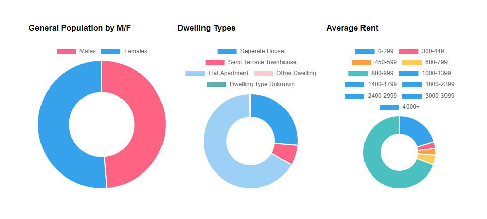
Yabber does a good job at returning basic donut graphs as the options are seriously limited (donut graphs are a one-dimensional rendering with a single data source). The following graphs of type language and citizen returns the following:

There is literally no end to the type of graphs you may create... and if advanced graphs are required, and Yabber doesn't support them, let us know and we'll build them in. The idea is that we'll have a 'Table Builder' built into Elementor that'll automatically render graphs of any type based on supplied attributes.

Census API

Making Simple Requests

The following function may be used to make simple requests. We're using the Requests library, although you could just as easily use PHP's file_get_contents() function.

<?php

Simple Census Request

function bm_get($url = '', $geo = '', $fields = '', $number = '') {

if ($url == '') return false;

if (strpos($url, 'https://') === false) $url = ENDPOINT . '?type=' . $url . '&code=' . $geo . '&fields=' . $fields . '&number=' . $number . '&apikey=' . APIKEY;

$response = WpOrg\Requests\Requests::get($url);

if ($response->status_code != 200) return false;

return json_decode($response->body, true);

}

The action, code, and fields values are the primary arguments used to return content. The action will determine what information is returned, while the code returns the type of geographic region we're querying, such as a postal code, electoral area, state, or other statistical area. In most cases on your website you will use a 4-digit numeric postcode.

The standard JSON response includes a ~~little~~ lot more detail than what might be considered necessary, and this is done to ensure that sufficient data is returned to make it easy to plugin into a graphing applications. The response usually includes a graph and labels key containing values that can be plugged directly into ChartJS or other graphing applications.

Details Endpoint

In many of our demos, we've used multiple statistical areas for the purpose of building comparison graphs. When any area is selected, you'll often want to automata the inclusion of 'nearby' postal areas, and the 'defaults' endpoint returns this (and other) data based on a single statistical area.

Note: We're provided a large number of postcode API resources in the past, such as the standard API, the Postcode Risk API, and others. Our free mortgage broker website plugin includes various geographic tools, and our property database is predicated on postal boundaries, so they're important assets that support our broader data engines. Despite all those tools serving valid functions, they will progressively be replaced by a newer API to consolidate our various resources.

When unwrapped, the returned details array includes the nearest 20 postal areas with distance and direction (more if required), schooling, hospital, POI, school, childcare, bank branch, ATM, hospital and care provider info - it's very extensive. General postal data and relevant geographic information is also returned.

Other Graphing Tools

The mortgage broker website we provide clients includes dozens of graphing tools, including RBA cash rate graphs, currency conversion graphs, and inflation graphs. The Yabber plugin also includes a means to manufacture your own line and bar graphs on the basis of shortcode (this will also be made into an Elementor plugin).

RBA Cash Rate: 4.35% · 1AUD = 0.67 USD · Inflation: 4.1%

Other Graphs: Shown is the RBA Graph, Currency Exchange Graph, and Comparison Rate graph. The shortcode used to render the rate graph was [bm_cashrate_graph points="800" start="20000101" rates_new_oo="0" rates_existing_oo="0" rates_investment="0" points="1000" height="450"] (so various options apply). We also used the shortcode of [show_cashrate_exchange] between the two graphs - used in the header of our broker website, but the attributes are available anywhere (of course, the individual values may be used anywhere with their own shortcode).

Considerations

Most graphs are a static resource. Once requested, they'll be cached in your 'saturn' cache for what is essentially forever. To clear the Saturn cache, you should do so in Yabber (this will refresh all Saturn data - not just graphs).
We index virtually every source of data the ABS releases (or we try to). As a result of potential confusion with shortcode, the Elmendor plugin will likely be the primary source to add new graphs.
The early Elementor Census plugin is made available only to very limited clients. Given the complexity of building a plugin that potentially returns hundreds of millions of graphs, we have no date for the Release Candidate.
Core Saturn integration will possibly be built into your website as early as next week. Over 2600 pages will be created regardless of whether you're partaking in the program. Note that for comparative purposes, all nearby geographic statistical areas will automatically be applied. It's expected that each page will include around 40 graphs. Keep in mind that having the pages isn't enough - you'll need to engage with the relationship program for the module to return results.
Values are returned from the 2021 Census so the data is a little out-of-date. Other more up-to-date sources are available. Another graph returns a range of rent for different dwelling types. Older Census sources are available for time-based comparisons.

Conclusion

An understanding of your audiences is a marketing and business imperative. Our Census API provides a double-edged advantage in that the information will be used to assess the suitability of various campaigns, but the graphing components on your website demonstrates a clear expertise and authoritativeness to your audiences. It's the 'lots of little things' that add up to a big thing.

With the introduction of some improvements to our system, our managed article program will include integrated graphing data as a priority.

Version 1 API: Version 1 of the Census API will continue to operate as always. Note that the update includes a new URL endpoint, but the request format remains unchanged.

Featured Image: A Census collector on horseback, 1911. Mr, R, B. Pitt (Charters Towers) will cover around 700 square miles of country. The gentleman standing is Mr. Frank Hasier, lands survuyer. The first population counts in Australia were made as early as 1788. From 1795 to 1825, ‘musters’ were held regularly where all members of the community gathered at specified locations to be counted. In 1828, the first colonial Census was conducted in New South Wales, with Tasmania in 1841, South Australia in 1844, Western Australia in 1848, and Victoria in 1854. In 1881, the first simultaneous Censuses of all the Australian colonies was conducted. In 1911, the first national Census was conducted by the Australian Bureau of Statistics (ABS). Around 7,300 people were appointed for the collection work. Field Officers travelled by horse, cart and bicycle to collect forms across the country and the information gathered was tabulated by hand. The Census was repeated in 1921, 1933, 1947, 1954, 1961, 1966 and from then on, every five years. In 1921, Census information was tabulated using mechanical machine equipment. The machines used in 1961 were so large that when delivered they could not fit through the door of the Census office in Canberra. A large hole had to be cut in the side of the wooden building to install them. The 1961 Census was the last to use tabulating machines.In 1954, women were hired to process and code data for the first time. The 1967 Referendum mandated all Aboriginal and Torres Strait Islander peoples be counted in the Australian Census. Computer technology was first used to process Census information in 1966 and people were provided with the option to complete their Census online in 2006. image Source: The Brisbane Courier 1 April 1911 p.13. Text Source: ABS.gov.au. [ View Image ]

Download our 650-page guide on Finance Marketing. We'll show you exactly how we generate Billions in volume for our clients.